Intro

Recently I worked on a document search for my current company. As part of the crawling and indexing process I worked on scoring the documents. The project was done during a hack week, and thus the scope was limited to what you can achieve in a few days. Because of that we started with a trivial approach and incrementally improved it from there on.

V1: Most trivial Approach

Concept: To score a document for a given query, we create a vector of all possible words (e.g. all the union of all unique words in all documents) and define this as our alphabet of size N. Next we define a function function c as c(w,q) ε {0|1} and c(w,d) ε {0|1}, which returns 0 or 1 based whether the given term w is in the given query resp. the given document.

We can think about this, as creating two bit vectors of size N. One document vector and one query vector. And then we can compute the score simply as the dot product of the two vectors.

This can also be expressed with Sum notation:

Naiv sum of occurrences

Over all possible words w(i) to w(N) we compute c(w,q) and c(w,d) and multiply the result. This means if the term is not present in the query or in our document, the product is 0 which is the identity / neutral element for sums. Then we just sum all these products.

Solved problems:

• score for matches
• no score for non matches

Open problems: If c(w,d) results in x, where x ε {0|1}, then the similarity of the document and query, is not expressed strong enough. With other words: Our score of 1/0 for matches is too simple to make a statement about how good a term in the query matches a given document. We can only say that it occurred at least once.

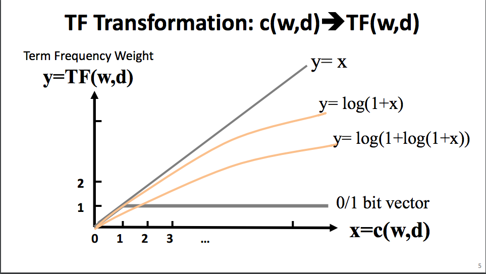
V2: Term frequency instead of a bit vector

Improvement: Instead of returning 0 or 1 for each possible word (bit vector), we return the count of occurrences of the given term. This is called the Term frequency (TF). So our counting function c is now defined as:

c(w,q) and c(w,d) = x , x >= 0

Solved problems:

• higher score for more matches
• no score for non matches
• c(w,d) now expresses the similarity of the word and the document better

Open problems:

• The frequency does not have an upper bound, so repeating the same word over and over again results in huge scores, thus we can have bad matches or people can fool our search engine
• Stop words and rare words have the same impact for the scoring function, thus words with a lot of regular english words but without any matches for nouns and verbs might score very high.

V3: Inverse Document frequency

Prioritize rare terms to common terms by introducing document frequency

In order to increase the importance of rare (meaningful) terms compared to common terms (stop words) we will penalize terms with occur in many documents (high document frequency). Therefore we can define:

M = Total number of all documents

and document frequency:

df(w) = number of documents that contain w

This approach is based on the idea of term specificity.

Now we can represent the inverse document frequency of w as:

inverse document frequency

Leading us to this new scoring function:

document frequency

With c(w,q) and c(w,d) = x , x >= 0

Solved problems:

• score for matches
• no score for non matches
• c(w,d) now expresses the similarity of the word and the document better
• rare terms are more important than stop words

Open problems:

• Term frequency does not have an upper bound, so repeating the same word over and over again results in huge scores.

V4: An upper bound for the Term frequency

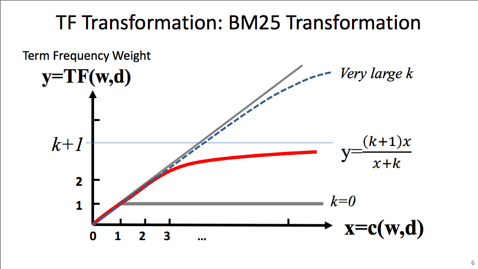
In order to address the final open issue lets take a look at BM25 as one of the available options to ensure an upper bound on the term frequency.

TF transformation BM25

BM25 is a well established algorithm for this task. It also falls back to our initial binary 1/0 logic for k = 0.

Using our c(w,d) as the x in the BM25 definition we just need to change one part of our scoring function and keep c(w,q) as well as the IDF term at the end. Our new equation looks like this:

New equation including BM25

Solved problems:

• higher score for more matches
• no score for non matches (multiplying query count by document count)
• c(w,d) now expresses the similarity of the word and the document better
• rare terms are more important than stop words (IDF)
• Term frequency has an upper bound so that repeating a single world many times does not fool our algorithm.

Open problems:

• When handling documents with different length, the longer documents will always have an advantage, since they have more content and are thus more likely to define the word we search for.

V5: Introduce Pivoted length normalization

Introducing document length normalization

To solve the final problem we are left with we will introduce a way to penalize very long documents to a certain degree to have a better balance for long and short documents. We define a “Normalizer” as follows:

Pivoted document length normalizer

with b ε [0,1]. Here b controls the impact of the normalizer. With b = 0 the normalizer is always 1, when we increase b towards 1 the penalty gets bigger.

We can now replace the simple use of k in our denominator with this normalizer, which us to our final equation.

New scoring function including document length normalizer

Solved problems:

• score matches
  • use of the sum of products
• do no score non matches
  • multiplication of query count by document count
• c(w,d) expresses the similarity of the term and the document
  • we replaced a bit vector with term frequency (TF)
• rare terms are more important than common words (stop words)
  • we added IDF
• Upper bound for term frequency, to handle repeated words properly
  • we added BM25
• handle a mix of short and long documents well
  • Introduction of document length normalization

Summary

We were able to arrive at a state of the art scoring function by incrementally improving our initial approach that was very naive and simple to implement. The similarity to the okapi / BM25 family can be compared in this wiki page or in the publications from Robertson and Walker about Okapi / BM25.

This article used equations based on the “vector space model”, which for example is used in Apache Lucene and which is quiet impressive this means even Elasticsearch used it under the hood! However other real world engines and the “official” BM25 definition uses a propabilistic relevance models instead. So maybe this might a interesting for futher reading.